[Python] Google Search Trend

Python에선 구글의 검색 트렌드를 분석할 수 있도록 pytrends라는 라이브러리를 제공한다.

시간순 선그래프

from pytrends.request import TrendReq
import matplotlib.pyplot as plt
import os

keyword = "space x"
period = "today 3-m"   

trend_obj = TrendReq()
trend_obj.build_payload(kw_list=[keyword], timeframe=period)

trend_df = trend_obj.interest_over_time()
print(trend_df.head())

plt.style.use("ggplot")
plt.figure(figsize=(14,5))
trend_df[keyword].plot()
plt.title("Google Trends over time", size=15)
plt.legend(labels=[keyword], loc="upper right")

cwd = os.getcwd()
output_filepath = os.path.join(cwd, ".", "google_trend_over_time_%s.png" % keyword)
plt.savefig(output_filepath, dpi=300)
plt.show()

10.1 Practical use_1 – Jupyter Notebook

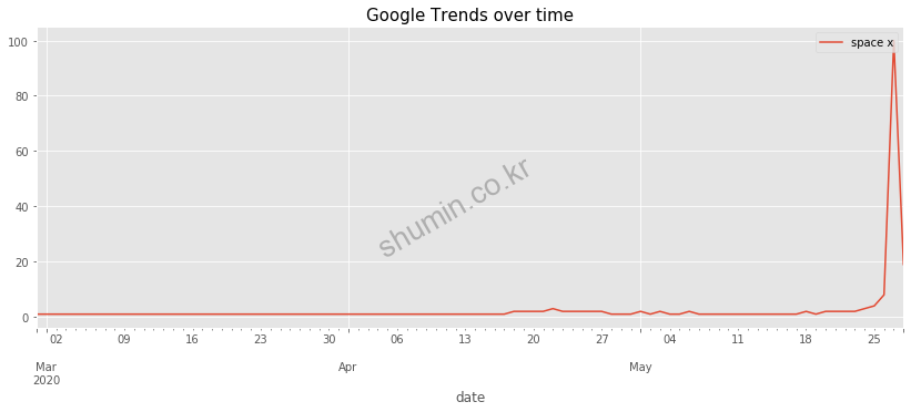
build_payload(kw_list=[keyword], timeframe=[period])과 trend_df = trend_obj.interest_over_time()를 통해 우리가 원하는 data를 data frame 형태로 받아 올 수 있다. (시간순으로)

지역별 막대그래프

아래 결과는 ‘WHO’의 검색에 대한 각 지역별로 어떻게 트렌드가 형성되는지 분석하는 코드다.

from pytrends.request import TrendReq
import matplotlib.pyplot as plt
import os

keyword = "WHO"
period = "now 7-d"   

trend_obj = TrendReq()
trend_obj.build_payload(kw_list=[keyword], timeframe=period)

trend_df = trend_obj.interest_by_region().sort_values(by='WHO', ascending=False)
print(trend_df.head())

plt.style.use("ggplot")
plt.figure(figsize=(14,10))
trend_df.iloc[:50, :][keyword].plot(kind='bar')
plt.title("Google Trends by Region", size=15)
plt.legend(labels=[keyword], loc="upper right")

cwd = os.getcwd()
output_filepath = os.path.join(cwd, ".", "google_trend_by_region_%s.png" % keyword)
plt.savefig(output_filepath, dpi=300)
plt.show()

trend_obj.interest_by_region().sort_values(by='WHO', ascending=False)를 통해 특정 지역별 검색 트렌드를 분석해 data frame으로 값을 얻을 수 있다.

최종 결과는 현재 업로드가 되지 않지만 각 나라별 검색 횟수에 대해 normalized value를 그래프로 보여준다.